

Sampling Path Candidates with Machine Learning#
This notebook aims to be a tutorial for reproducing the results presented in the paper Transform-Invariant Generative Ray Path Sampling for Efficient Radio Propagation Modeling, and assumes you are familiar with its content.
Important
This notebook presents version 2 of our work on the topic of sampling path candidates. You can access v1, as presented at the 2025 IEEE International Conference on Machine Learning for Communication and Networking (ICMLCN) in our paper Towards Generative Ray Path Sampling for Faster Point-to-Point Ray Tracing [3] by clicking here.
You can run it locally or with Google Colab by clicking on the rocket at the top of this page!
Tip
On Google Colab, make sure to select a GPU or TPU runtime for a faster experience.
If you find this tutorial useful and plan on using this tool for your publications, please cite our work; see Citing.
Warning
Training the models can take quite some time.
If you want to bypass the training and use a pre-trained model,
you can download the weights from the
releases page and
load them with Model.load_weights.
Summary#
In our work, we present a machine learning model that aims to reduce the computational complexity of exhaustive point-to-point Ray Tracing by learning how to sample path candidates. For further details, please refer to the paper.
Setup#
Below are the important steps to properly set up the environment.
Imports#
Unlike for the previous version of our work, we have refactored the codebase to be more modular and reusable.
This means that most of the code is located in separate files,
available on GitHub,
and installed as a Python package (sampling_paths).
This notebook is meant to be a tutorial on how to use the package to train and use the model, and thus does not contain the implementation details of the model itself.
We need to import quite a few Python modules,
but all of them should be installed with
pip install --group notebooks git+https://github.com/jeertmans/sampling-paths.git
(assuming pip >= 25.1).
The following cell is hidden by default for readability.
Pretty Printing#
Nested structures, like machine learning modules, or more generally PyTrees, do not render very nicely by default.
To provide the user with an interactive pretty-printing experience, we use treescope:
treescope.basic_interactive_setup()
JAX Device#
While this notebook will run fine on all supported JAX devices (i.e., CPU, GPU, and TPU), using a GPU (or a TPU) will usually decrease the computational time by a significant factor.
To check the currently active JAX device, use jax.devices:
jax.devices()
Generating the training data#
For this tutorial, as in the paper, we restrict ourselves to a simple urban scenario, obtained from Sionna [9], from which we will derive random scenes.
download_sionna_scenes() # Let's download Sionna scenes (from the main branch)
set_defaults(
"plotly"
) # Our scene is simple, and Plotly is the best backend for online interactive plots :-)
def make_transparent(fig: go.Figure) -> go.Figure:
fig.update_scenes(
xaxis_visible=False, yaxis_visible=False, zaxis_visible=False
)
return fig
fig = BASE_SCENE.plot()
make_transparent(fig)
From the BASE_SCENE object, we can generate random variations of it.
Two main types of variations are considered here:
the number of objects (either triangles or quadrilaterals);
and the TX / RX positions.
Note
Unlike with NumPy and other common array libraries,
JAX requires an explicit random key (jr.key) whenever you need to generate
pseudo-random numbers. While this can lead to more verbose code, this has the
major advantage of making random number generation easily reproducible,
even across multiple devices. You want the same results? Then just pass the same key!
Below, we demonstrate how to generate (and plot) a random scene.
example_scene = random_scene(sample_in_canyon=True, key=jr.key(1234))
example_fig = example_scene.plot(
showlegend=False,
tx_kwargs={"labels": ["TX"]},
rx_kwargs={"labels": ["RX"]},
mesh_kwargs={"opacity": 0.5},
)
make_transparent(example_fig)
In the paper, we study other types of random variations,
and they can be specified with optional parameters of the random_scene function.
help(random_scene)
Help on _JitWrapper in module sampling_paths.utils:
random_scene(*, min_fill_factor: float = 0.5, max_fill_factor: float = 1.0, tx_z_min: float = 2.0, tx_z_max: float = 50.0, rx_z_min: float = 1.0, rx_z_max: float = 2.0, sample_objects: bool = True, sample_in_canyon: bool = True, include_floor: bool = True, key: Union[jaxtyping.Key[jaxlib._jax.Array, ''], jaxtyping.UInt32[jaxlib._jax.Array, '2']]) -> differt.scene._triangle_scene.TriangleScene
Return a random scene with one TX and one RX, at random positions, and a random number of objects.
The number of objects is randomly sampled based on a random fill factor.
Args:
min_fill_factor: The minimum fill factor to be used.
max_fill_factor: The maximum fill factor to be used.
tx_z_min: Minimum height of the transmitter.
tx_z_max: Maximum height of the transmitter.
rx_z_min: Minimum height of the receiver.
rx_z_max: Maximum height of the receiver.
sample_objects: Whether to sample objects in the scene, instead of individual primitives.
sample_in_canyon: Whether to sample the TX and RX positions within the canyon area.
include_floor: Whether to always include the floor in the scene.
key: The random key to be used.
Returns:
A new scene.
Afterward, we can trace ray paths in the generated scene and plot them.
with reuse(figure=example_fig) as fig:
num_active_primitives = example_scene.mesh.num_active_primitives
for order in [0, 1, 2, 3]:
num_valid_paths = 0
if order == 0:
num_path_candidates = 1
else:
num_path_candidates = num_active_primitives * (
num_active_primitives - 1
) ** (order - 1)
for paths in tqdm(
example_scene.compute_paths(order=order, chunk_size=1_000_000),
desc="Processing path candidates",
leave=False,
):
num_valid_paths += paths.num_valid_paths
paths.plot(showlegend=False)
print(
f"(order = {order}) Found {num_valid_paths:2d} valid paths out of {num_path_candidates:6d} path candidates."
)
fig
(order = 0) Found 1 valid paths out of 1 path candidates.
(order = 1) Found 2 valid paths out of 62 path candidates.
(order = 2) Found 1 valid paths out of 3782 path candidates.
(order = 3) Found 1 valid paths out of 230702 path candidates.
We then collect some statistics about the scenes we will be training on.
Note
Unlike with the example scene, the training set will include TX and RX positions outside the main street canyon.
You can override this by modifying the parameters passed to the train_dataloader and scene_fn functions when instantiating the Agent object.
# Keyword parameters passed 'train_dataloader' and the agent's 'scene_fn' function.
scene_fn_kwargs = {"sample_in_canyon": False}
scenes = train_dataloader(key=jr.key(1234), **scene_fn_kwargs)
num_valid_paths = defaultdict(list) # Number of valid paths
num_total_paths = defaultdict(list) # Total number of paths (candidates)
colors = {0: "black", 1: "blue", 2: "red", 3: "green"}
for _ in trange(
10_000,
desc="Collecting statistics over many realizations",
leave=False,
):
scene = next(scenes)
num_active_primitives = scene.mesh.num_active_primitives
for order in colors:
num_valid_paths[order].append(0)
if order == 0:
num_path_candidates = 1
else:
num_path_candidates = num_active_primitives * (
num_active_primitives - 1
) ** (order - 1)
num_total_paths[order].append(num_path_candidates)
for paths in scene.compute_paths(order=order, chunk_size=100_000):
num_valid_paths[order][-1] += paths.mask.sum()
fig = go.Figure()
for order, color in colors.items():
print(f"\tStatistics for {order = }:")
num_valid = jnp.array(num_valid_paths[order])
num_total = jnp.array(num_total_paths[order])
where = num_total != 0 # We discard rare cases without any candidate
avg_total = int(num_total.mean(where=where))
frac = float((num_valid / num_total).mean(where=where))
frac_one = float((num_valid > 0).sum(where=where) / where.sum())
print(
f"\t- an average of {avg_total} path candidates exist;\n"
f"\t- out of which {frac:.8%} of the paths are valid\n"
f"\t- and {frac_one:.8%}% of the scenes contained at least one valid path."
)
fig.add_histogram(
x=num_valid,
histnorm="percent",
name=f"{order = }",
marker_color=color,
)
fig.update_layout(
title="Distribution of the number of valid ray paths per scene",
xaxis_title="Number of valid paths",
yaxis_title="Percentage of scenes (%)",
)
Statistics for order = 0:
- an average of 1 path candidates exist;
- out of which 34.15000141% of the paths are valid
- and 34.15000141%% of the scenes contained at least one valid path.
Statistics for order = 1:
- an average of 56 path candidates exist;
- out of which 1.46392491% of the paths are valid
- and 37.62000203%% of the scenes contained at least one valid path.
Statistics for order = 2:
- an average of 3365 path candidates exist;
- out of which 0.02076994% of the paths are valid
- and 24.73000139%% of the scenes contained at least one valid path.
Statistics for order = 3:
- an average of 211723 path candidates exist;
- out of which 0.00033600% of the paths are valid
- and 12.03000024%% of the scenes contained at least one valid path.
Reward function#
As for every reinforcement learning problem, we need to define a reward function that will guide the training of our model.
Here, we use a binary reward function that indicates if a generated path candidate leads to a valid ray path or not.
When computing paths with
TriangleScene.compute_paths,
assuming default parameters,
the Paths.mask attribute
is a boolean array where each entry indicates if the corresponding ray
path is valid or not. As we only have one pair of TX and RX, the sum
of all entries in this mask, when converted to floating point values,
is either 1 or 0. This will be our reward.
The default reward function can be imported with:
from sampling_paths.metrics import reward_fn
Differentiable reward#
As differt is a differentiable library, thanks to JAX,
the reward function will be differentiable with respect to its arguments.
Simulating non-differentiable reward#
In our previous work, we already observed that using a non-differentiable reward leads to worse training performance.
To observe this effect, you can use jax.lax.stop_gradient
to prevent gradients from flowing through the reward function.
To do so, when creating the model (see below), pass the following reward function:
Model(
...,
reward_fn=lambda path_candidate, scene: jax.lax.stop_gradient(
reward_fn(path_candidate, scene)
),
)
Machine Learning model#
Our model is made of four modules: an outer flow model that returns the flows between a parent state and its child states, and three inner models, each encoding different aspects of the scene.
The model’s internals are detailed in the paper and will not be discussed here.
Below, we instantiate the model with default parameters.
order = 2 # Change this to try different path orders
num_embeddings = 128
model = Model(
order=order,
num_embeddings=num_embeddings,
width_size=2 * num_embeddings,
depth=2,
key=jr.key(1234),
)
model
Training with an agent#
To train the model, we define an agent that will handle the training loop for us.
This is mainly syntactic sugar to avoid writing boilerplate code, as the agent does not add any new functionality to the model itself.
Instead, it provides a convenient interface to train the model over multiple epochs,
track metrics, and alternate between the standard training step and the replay buffer training step, which are automatically handled by the agent’s train method.
To optimize the model’s parameters, we rely on the optax module that provides
convenient optimizers, from which we use the optax.contrib.muon optimizer.
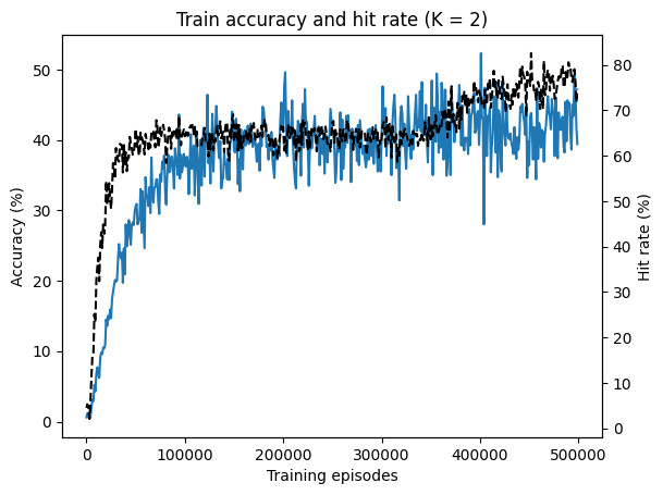
Every few training steps, we will ask the agent to evaluate the model’s performance to obtain the curves presented in the paper.
class Results(eqx.Module):
episodes: Int[Array, " n"]
loss_values: Float[Array, " n"]
success_rates: Float[Array, " n"]
hit_rates: Float[Array, " n"]
fill_rates: Float[Array, " n"] | None
def train(
model: Model,
*,
num_validation_scenes: int = 100,
num_episodes: int = 500_000,
evaluate_every: int = 1_000,
key: PRNGKeyArray,
) -> tuple[Model, Results]:
key_episodes, key_valid_samples = jr.split(key)
valid_keys = validation_scene_keys(
order=model.order,
num_scenes=num_validation_scenes,
key=key_valid_samples,
**scene_fn_kwargs,
)
agent = Agent(
model=model,
scene_fn=partial(random_scene, **scene_fn_kwargs),
)
episodes = []
loss_values = []
success_rates = []
hit_rates = []
fill_rates = []
progress_bar = tqdm(
jr.split(key_episodes, num_episodes), desc="Training model"
)
for episode, key_episode in enumerate(progress_bar):
scene_key, train_key, eval_key = jr.split(key_episode, 3)
# Train
agent, loss_value = agent.train(scene_key, key=train_key)
# Evaluate
if episode % evaluate_every == 0:
accuracy, hit_rate = agent.evaluate(valid_keys, key=eval_key)
progress_bar.set_description(
"Training model - "
f"loss: {loss_value:.1e}, "
f"success rate: {accuracy:.2%}, "
f"hit rate: {hit_rate:.2%}"
+ (
f", buffer filled: {agent.replay_buffer.fill_ratio:.2%}"
if agent.replay_buffer is not None
else ""
),
)
episodes.append(episode)
loss_values.append(loss_value)
success_rates.append(100 * accuracy)
hit_rates.append(100 * hit_rate)
if agent.replay_buffer is not None:
fill_rates.append(100 * agent.replay_buffer.fill_ratio)
results = Results(
episodes=jnp.asarray(episodes),
loss_values=jnp.asarray(loss_values),
success_rates=jnp.asarray(success_rates),
hit_rates=jnp.asarray(hit_rates),
fill_rates=jnp.asarray(fill_rates) if fill_rates else None,
)
return eqx.nn.inference_mode(agent.model), results
trained_model, results = train(model, key=jr.key(1234))
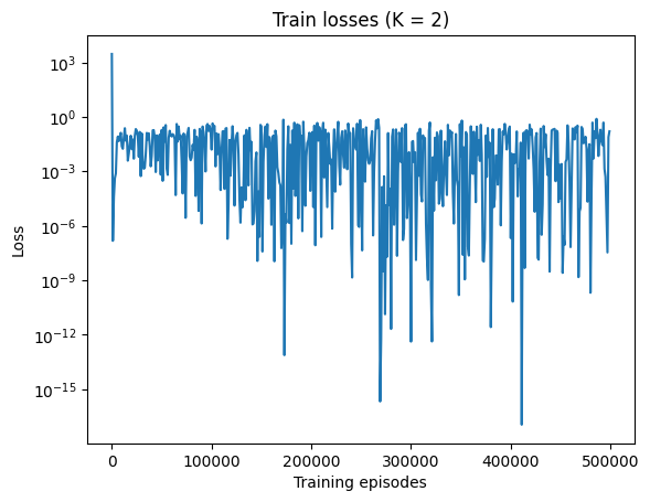
plt.figure()
plt.title(f"Train losses (K = {order})")
plt.semilogy(results.episodes, results.loss_values)
plt.xlabel("Training episodes")
plt.ylabel("Loss")
plt.show()
_, ax1 = plt.subplots()
ax1.set_title(f"Train accuracy and hit rate (K = {order})")
ax1.set_xlabel("Training episodes")
ax1.set_ylabel("Accuracy (%)")
ax1.plot(results.episodes, results.success_rates, label="Accuracy")
ax2 = ax1.twinx()
ax2.set_ylabel("Hit rate (%)")
ax2.plot(results.episodes, results.hit_rates, "k--", label="Hit Rate")
plt.show()
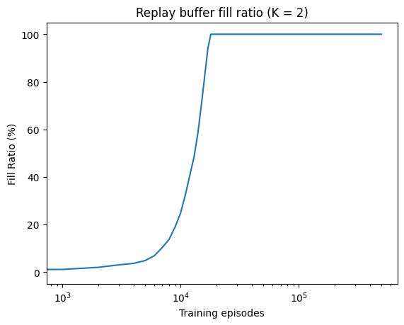
if results.fill_rates is not None:
plt.figure()
plt.title(f"Replay buffer fill ratio (K = {order})")
plt.semilogx(results.episodes, results.fill_rates, label="Fill Ratio")
plt.xlabel("Training episodes")
plt.ylabel("Fill Ratio (%)")
plt.show()
trained_models = {trained_model.order: trained_model}
save_weights = True
for order in tqdm([0, 1, 2, 3], desc="Orders"):
if order in trained_models:
continue
model = Model(
order=order,
num_embeddings=num_embeddings,
width_size=2 * num_embeddings,
depth=2,
key=jr.key(1234),
)
if order > 0:
trained_model, _ = train(model, key=jr.key(1234))
else:
# No need to train LOS model
trained_model = eqx.nn.inference_mode(model)
trained_models[order] = trained_model
if save_weights:
for order, trained_model in trained_models.items():
if order == 0:
continue # Don't save line-of-sight model
with open(f"model_{order}.eqx", "wb") as f:
eqx.tree_serialise_leaves(f, trained_model)
Using the model for coverage map estimation#
def compute_cm(
receivers: Float[Array, "dim_x dim_y 3"],
base_scene: TriangleScene,
model: Model,
batch_size: int,
key: PRNGKeyArray | None,
) -> Float[Array, "dim_x dim_y"]:
# N.B.: we use sequential_vmap to avoid out-of-memory errors in the exhaustive case
@jax.custom_batching.sequential_vmap
def compute_cm_for_one_receiver(
receiver: Float[Array, "3"],
) -> Float[Array, ""]:
scene = eqx.tree_at(lambda s: s.receivers, base_scene, receiver)
if key is not None and model.order > 0:
path_candidates = jax.vmap(lambda key: model(scene, key=key))(
jr.split(key, batch_size)
)
paths = scene.compute_paths(path_candidates=path_candidates)
paths = (
paths.mask_duplicate_objects()
) # Important to remove duplicate path candidates
else:
# Exhaustive method does not contain duplicate path candidates
paths = scene.compute_paths(order=model.order)
r = path_lengths(paths.vertices)
e = safe_divide(1.0, r)
return (e * e).sum(where=paths.mask)
return jax.vmap(jax.vmap(compute_cm_for_one_receiver))(receivers)
M = 10
batch = (300, 300)
z0 = 1.5
base_scene = eqx.tree_at(
lambda s: s.transmitters, BASE_SCENE, jnp.array([[0.0, 0.0, 32.0]])
)
receivers = base_scene.with_receivers_grid(*batch, height=z0).receivers
# Only needed for plotting purposes
x, y, _ = jnp.unstack(receivers, axis=-1)
fig = make_subplots(
rows=1,
cols=2,
specs=[[{"type": "scene"}, {"type": "scene"}]],
)
with reuse(figure=fig) as fig:
base_scene.plot(
tx_kwargs={"marker_color": "#636EFA"}, showlegend=False, row=1, col=1
)
base_scene.plot(
tx_kwargs={"marker_color": "#636EFA"}, showlegend=False, row=1, col=2
)
G_model = G_exhau = jnp.zeros(batch)
for order in [0, 1, 2, 3]:
G_model += compute_cm(
receivers, base_scene, trained_models[order], M, jr.key(0)
)
G_exhau += compute_cm(
receivers, base_scene, trained_models[order], 0, None
)
G_min = jnp.minimum(G_model.min(), G_exhau.min())
G_max = jnp.maximum(G_model.max(), G_exhau.max())
draw_image(
10 * jnp.log10(G_model),
x=x[0, :],
y=y[:, 0],
z0=z0,
colorbar={"title": "Gain (dB)"},
colorscale="viridis",
cmin=float(10 * jnp.log10(G_min)),
cmax=float(10 * jnp.log10(G_max)),
row=1,
col=1,
showscale=False,
)
draw_image(
10 * jnp.log10(G_exhau),
x=x[0, :],
y=y[:, 0],
z0=z0,
colorbar={"title": "Gain (dB)"},
colorscale="viridis",
cmin=float(10 * jnp.log10(G_min)),
cmax=float(10 * jnp.log10(G_max)),
row=1,
col=2,
)
fig